Torque / Force Controller#
The Torque / Force controller is an implementation where, based on the measurement of the external forces and torques, the system adjusts the actuator commands to achieve or maintain a desired force or torque profile.
1. Overview & Control Architecture#
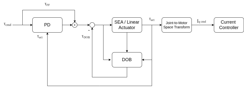
The torque/force controller operates inside the Field Oriented Control (FOC) loop. It regulates the force (for linear joints) or torque (for rotational joints) acting on the output joint. The control architecture is composed of three primary pathways:
Feedforward Path (\(u_{\text{ff}}\)): Direct injection of the desired joint force reference to improve tracking responsiveness and reduce phase lag.
Feedback PD Path (\(u_{\text{PD}}\)): Proportional-Derivative (PD) feedback based on the error between the desired force and the actual (measured) force, with low-pass filtering on the derivative term to mitigate noise.
Disturbance Observer (DOB) Path (\(U_{\text{dob}}\)): Active friction and disturbance compensation using a physics-based joint model. It calculates unmodeled loads (e.g., joint friction, external load variations) to dynamically correct the output effort.
The final joint-space command is converted back to motor space and sent as a current reference (\(i_q^*\)) to the FOC q-axis current PI controller.
The following schema illustrates the whole control loop:
2. Force & Torque Measurement Feedback#
To close the torque controller loop, the system requires real-time feedback of the interaction force/torque acting at the joint level. Depending on the mechanical design of the robot, this feedback is either measured directly using an output load cell, or estimated indirectly using the spring deflection of a Series Elastic Actuator (SEA).
2.1 Direct Force Sensing#
When the system is configured to use the force sensor, it interfaces with a physical strain-gauge load cell on the joint’s output stage via a sensor signal conditioner over the \(I^2C\) protocol. This signal, after some filtering and calibration adjustment (zero-offset subtraction and directional sensitivity scaling), is ready to be injected into the control loop.
2.2 Indirect Series Elastic Actuator (SEA) Estimation#
When configured as a Series Elastic Actuator, no physical load cell is used. Instead, a mechanical spring element with a known stiffness (\(K_{\text{jointStiffness}}\)) is situated between the motor gearbox and the output joint. By measuring the positional deflection across the spring, the joint torque is mathematically estimated.
3. Actuator Kinematics & Space Transformations#
To keep the control logic generic across different mechanical designs, the torque controller performs calculations in Joint Space using standard units Newtons (\(N\)). The transformation ratio \(R_{\text{motor2joint}}\) maps motor-space quantities (motor torque, motor inertia, rotor acceleration) to joint-space quantities.
3.1 Linear Joints#
For linear actuators driven by a lead screw, the motor torque is transformed into joint linear force based on the lead screw pitch:
Where \(p_{\text{pitch_mm}}\) is the lead screw pitch in millimeters. If the lead screw has a right-handed helix (or vice versa depending on configuration), the direction is inverted:
3.2 Rotational Joints#
For rotational actuators utilizing gear reduction, the motor torque is scaled directly by the reduction ratio:
3.3 Space-Transformed Rotor Inertia#
Accelerating the motor’s rotor requires inertial torque. This inertial torque must be accounted for and subtracted from the sensed force so the feedback loop responds purely to external loads. The rotor inertia reflected to the joint space (\(J_{\text{joint_inertia_effort}}\)) is calculated as:
Where \(J_{\text{motor}}\) is the physical rotor inertia of the motor and \(\alpha_{\text{motor}}\) is the actual motor acceleration.
4. Control Law Formulation#
The core control function executes the following algorithmic steps at each control cycle.
4.1 Input Limitation & Reference Feedforward#
The desired force/torque reference command \(F_{\text{desired}}\) is first clamped to ensure it does not exceed pre-configured safety bounds:
The baseline feedforward effort is initialized directly to this limited reference:
4.2 Proportional-Derivative (PD) Feedback Control#
The feedback error is computed as the difference between the desired force and the offset-corrected actual force:
Proportional Term (\(U_p\)):
\[ U_p = K_p \times e(t) \]Derivative Term (\(U_d\)): To prevent derivative kick from sensor noise, the raw derivative of the force feedback is computed via a backward difference scheme and then filtered through a dedicated low-pass filter:
\[\dot{F}_{\text{raw}}(t) = \frac{F_{\text{actual}}(t) - F_{\text{actual}}(t - \Delta t)}{\Delta t}\]\[\dot{F}_{\text{filtered}}(t) = \text{LPF}(\dot{F}_{\text{raw}})\]\[U_d = -K_d \times \dot{F}_{\text{filtered}}(t)\]
The combined feedback control output is:
4.3 Disturbance Observer (DOB)#
The Disturbance Observer estimates friction, gear inefficiencies, and unmodeled forces by examining the mismatch between expected joint efforts and actual sensed joint efforts.
Electromagnetic Effort Calculation: Rather than using the previous command target, the expected torque/force is computed directly from the actual measured motor phase current (\(I_{\text{actual}}\) in Amperes) scaled to joint space:
\[T_{\text{expected_joint}} = I_{\text{actual}} \times R_{\text{motor2joint}} \times K_t\]Raw Disturbance Estimation (\(\tau_{\text{dob}}\)): The disturbance is estimated by subtracting the joint-space rotor inertia effort and the actual measured force from this expected electromagnetic effort:
\[\tau_{\text{dob}} = T_{\text{expected_joint}} - J_{\text{joint_inertia_effort}} - F_{\text{actual}}\]Low-Pass Filtering: The raw estimate \(\tau_{\text{dob}}\) contains high-frequency noise from current sensing and numerical acceleration derivatives. It is filtered using the observer filter:
\[\tau_{\text{dob_filtered}} = \text{LPF}\left(\tau_{\text{dob}}\right)\]DOB Control Action (\(U_{\text{dob}}\)): The disturbance compensation term is scaled by the observer gain \(K_{\text{dob}}\):
\[U_{\text{dob}} = K_{\text{dob}} \times \tau_{\text{dob_filtered}}\]
5. Output Current Command & Constraints#
The combined joint-space control command \(u_{\text{cmd}}\) is the sum of the feedforward term, the PD feedback, and the DOB compensation:
5.1 Mapping to Motor Space Current#
To apply this command to the motor, the joint-space force/torque is mapped back to a motor-space q-axis current command (\(i_{\text{cmd}}\)) in Amperes:
5.2 Saturation and Safety Clamping#
Finally, to protect the motor windup, physical gearings, and driver stage, the current command is clamped to the maximum current controller limit: